No Frills Time Series Compression That Also Works

CSV + gzip will take you far. • August 22, 2023

So you have some time series data and you want to make it smaller? You may not need an algorithm designed specifically for time series. Generic compressors like gzip work quite well and are much easier to use.

Of course this depends on your data, so there’s some code you can use to try it out here.

Recently I started working on a way to save Bluetooth scale data in my iOS coffee-brewing app. I want to allow people to record from a scale during their coffee-brewing sessions and then view it afterwards. Scale data is just a bunch of timestamps and weight values. Simple, yes, but it felt like something that might take a surprising amount of space to save. So I did some napkin math:


                1 scale session / day
                

                10 minutes / session
                

                10 readings / second
                

                = 2.19M readings / year


                1 reading = 1 date + 1 weight
                

                = 1 uint64 + 1 float32
                

                = 12 bytes
                

                2.19M * 12B = 26 MB

26 MB per year is small by most measures. However in my case I keep a few extra copies of my app’s data around as backups so this is more like ~100MB/year. It’s also 40x the size of what I’m saving currently! This puts my app in danger of landing on the one Top Apps list I would not be stoked to be featured on:

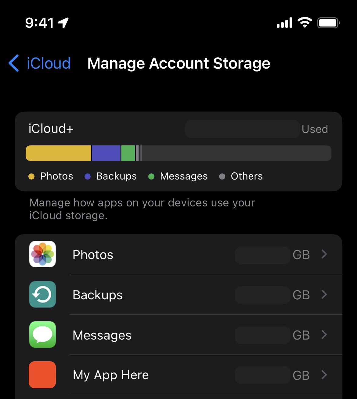_{iCloud storage usage}

So let’s avoid that. At a high-level I see two options:

Save less. 10 scale readings/second is probably more granularity than we’ll ever need. So we could just not save some of them. Of course if I’m wrong about that, they’re gone forever and then we’ll be out of luck.

Save smaller. Looking at some example data, there are a lot of plateaus where the same value repeats over and over. That seems like it could compress well.

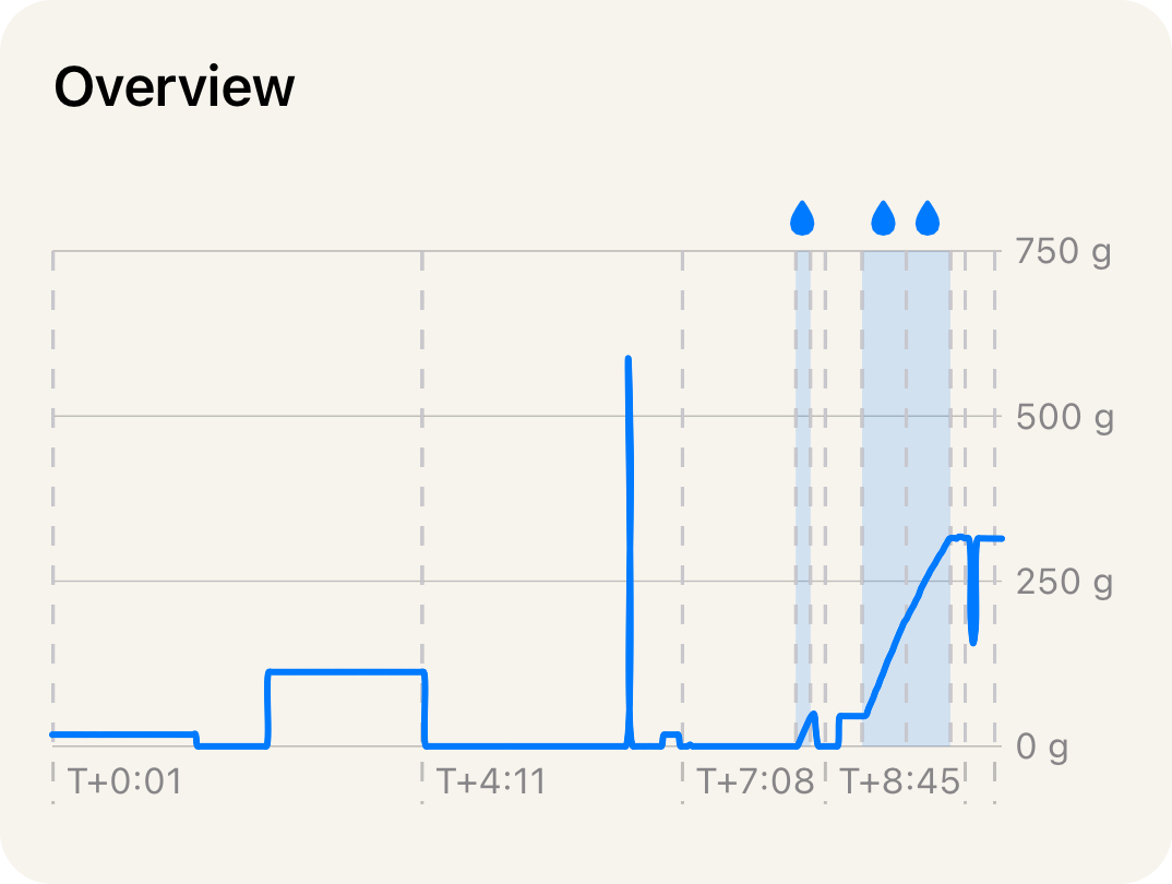_{Example brewing session time series}

Picking Ways to Compress

This is my first rodeo with compression. I’m starting from basics like “compression makes big things small” and “double click to unzip”. Doing a little research seems like a good idea and it pays off.

My scale data is technically “time series data” and it turns out we are not the first to want to compress it. There is a whole family of algorithms designed specifically for time series. This blog post is a great deep dive, but for our purposes today we’ll be looking at two of the algorithms it mentions:

simple-8b which compresses sequences of integers
Gorilla which compresses both integers as well as floating point numbers

Algorithms designed for exactly my problem space sound ideal. However something else catches my eye in a comment about the same blog post:

rklaehn on May 15, 2022
I have found that a very good approach is to apply some very simple transformations such as delta encoding of timestamps, and then letting a good standard compression algorithm such as zstd or deflate take care of the rest.

Using a general purpose algorithm is quite intriguing! One thing I’ve noticed is that there are no Swift implementations for simple-8b or Gorilla. This means I would have to wrap an existing implementation (a real hassle) or write a Swift one (risky, I would probably mess it up). General purpose algorithms are much more common and side-step both of those issues.

So we’ll look at both. For simplicity I’ll call simple-8b and Gorilla the “specialist algorithms” and everything else “generalist”.

Evaluating the Specialist Algorithms

Starting with the specialists seems logical. I expect they will perform better which will give us a nice baseline for comparison. But first we need to smooth out a few wrinkles.

Precision

While wiring up an open-source simple-8b implementation I realize that it requires integers and both our timestamp and weight are floating point numbers. To solve this we’ll truncate to milliseconds and milligrams. A honey bee can flap its wings in 5 ms. A grain of salt is approximately 1mg. Both of these feel way more precise than necessary but better to err on that side anyways.


                49.0335097 seconds
                

                17.509999999999998 grams


                49033 milliseconds
                

                17509 milligrams

We’ll use this level of precision for all our tests except Gorilla, which is designed for floating point numbers.

Negative Numbers

Negative numbers show up semi-frequently in scale data because often when you pick something up off a scale it will drop below zero.

Unfortunately for us simple-8b doesn’t like negative numbers. Why? Let’s take a little detour and look at how computers store numbers. They end up as sequences of 1s and 0s like:


            0000000000010110 is 22
            

            0000000001111011 is 123
            

            0000000101011110 is 350

You’ll notice that these tend to have all their 1s all on the right. In fact, only very large numbers will have 1s on the left. simple-8b does something clever where it uses 4 of the leftmost spaces to store some 1s and 0s of its own. This is fine for us. We’re not storing huge numbers so those leftmost spaces will always be 0 in our data.

Now let’s look at some negatives.


            1111111111101010 is -22
            

            1111111110000101 is -123
            

            1111111010100010 is -350

This is not great, the left half is all 1s! Simple-8b has no way of knowing whether the leftmost 1 is something it put there or something we put there so it will refuse to even try to compress these.

One solution for this is something called ZigZag encoding. If you look at the first few positive numbers, normally they’ll look like this:


            0000000000000001 is 1
            

            0000000000000010 is 2
            

            0000000000000011 is 3
            

            0000000000000100 is 4

ZigZag encoding interleaves the negative numbers in between so now these same 0/1 sequences take on a new meaning and zig zag between negative and positive:


            0000000000000001 is -1 zig
            0000000000000010 is  1 zag
            0000000000000011 is -2 zig
            0000000000000100 is  2 zag

If we look at our negative numbers from earlier, we can see that this gets rid of our problematic left-side 1s.

#	Normal	ZigZag
`-22 -123 -350`	`1111111111101010 1111111110000101 1111111010100010`	`0000000000101011 0000000011110101 0000001010111011`

We only need this for simple-8b, but it can be used with other integer encodings too. Kinda cool!

Pre-Compression

Technically we could run our tests now, but we’re going to do two more things to eke out a little extra shrinkage.

First is delta encoding. The concept is simple: you replace each number in your data set with the difference (delta) from the previous value.


                timestamp,mass
                

                1691452800000,250
                

                1691452800103,253
                

                1691452800305,279
                

                …

→


                timestamp_delta,mass_delta
                

                1691452800000,250
                

                103,3
                

                202,26
                

                …

Visually these already look smaller. Amusingly enough they actually are smaller. We’ll use this for all algorithms except Gorilla which does delta encoding for us.

The second tweak relates to the ordering of our data. So far we’ve been talking about time series as pairs of (timestamp, mass) points. Both specialist algorithms require us to provide a single list of numbers. We have two choices to flatten our pairs:


            Choice 1: [first_timestamp, first_mass, second_timestamp, second_mass, …]
            

            Choice 2: [first_timestamp, second_timestamp, … last_timestamp, first_mass, second_mass, …]

Choice 2 compresses better on all algorithms (generalist too) even when we apply it after delta encoding. Again, Gorilla does its own thing–are you seeing the trend?

Specialist Results

We’ve truncated and pre-encoded, so let’s see some results.

Algorithm	Ratio 1	Ratio 2	Ratio 3	Avg. Ratio	Avg. MB/year
simple-8b	6.92	5.4	7.18	6.5	4
gorilla	6.72	4.18	6.88	5.9	4.4
	⊢ higher is better ⊣				lower is better

I tested with three different types of scale recordings for a bit of variety, then backed out the MB/year from the average compression ratio. Going from 26 MB/year to under 5 is a great result!

Now for the Generalist Ones

Similar to the specialist algorithms, we have a few choices to make before we can run our tests on the generalists.

Formatting

For simplicity we’re going to format our data as CSV. This might seem a little odd but it has a few perks:

It’s human-readable which is nice for debugging.
It’s also fairly compact as far as text representations go.
Most languages have native libraries to make reading/writing CSVs easy. ^{(alas,
Swift does
not)}

We’ll use delta encoding like above–it’d be silly not to. We could really stretch the definition of CSV and stack all of the timestamps on top of all the masses into a single column, but that sacrifices a bit of readability so we won’t.

Picking Algorithms

There are a lot of general purpose compression algorithms. One popular benchmark lists over 70! We’re going to pick just 5. They are:

zlib, LZMA, and LZFSE – these come built-in with iOS which makes my life easier. zlib and LZMA are also fairly common.
Zstandard (aka zstd) and Brotli – from Facebook and Google respectively, both companies with an interest in good compression

Picking Levels

We’ve narrowed it down from 70 to 5, but there’s another curveball. Unlike the specialist algorithms which have no configuration options, most generalist algorithms let you choose a level that trades off speed for better compression. You can compress fast or slow down to compress more.

For simplicity (and so I don’t have to show you a table with 40+ rows) we are not going to test all 11 Brotli levels or all 20+ zstd levels. Instead we’re going to choose levels that run at about the same speed. Apple makes this easier for us since LZFSE has no level and iOS only has zlib 5 and LZMA 6. All we have to do is pick levels for Brotli and zstd from this chart.

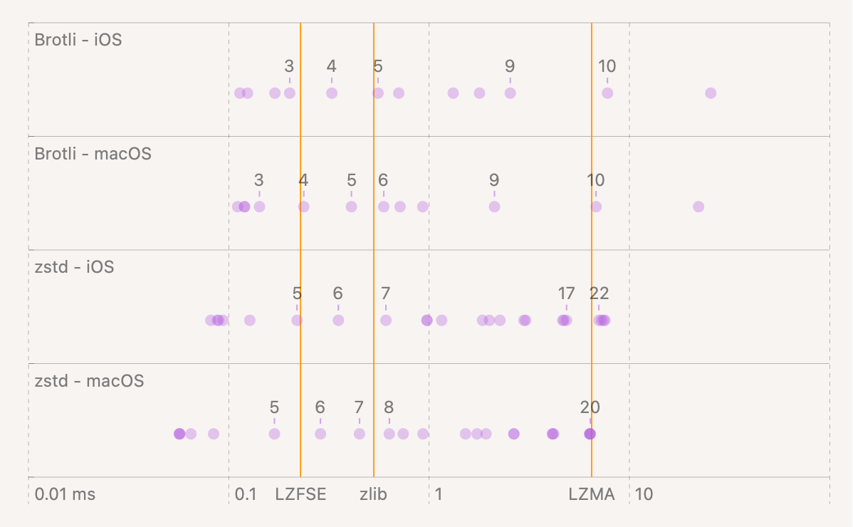_{Speed benchmarks for our 5
algorithms}

We’ll use Brotli 4 and zstd 5 since those are in-line with the fastest iOS algorithm. This means that zlib and LZMA are slightly advantaged but we’ll keep that in mind.

Generalist Results

We’ve prepped our CSV and made all our choices, so let’s see some results.

Algorithm	Ratio 1	Ratio 2	Ratio 3	Avg. Ratio	Avg. MB/year
zlib 5	8.50	5.79	8.18	7.49	3.47
lzma 6	8.12	5.55	7.49	7.1	3.7
zstd 5	7.49	5.71	7.74	6.98	3.72
brotli 4	7.84	5.52	7.53	6.96	3.74
lzfse	7.49	5.36	7.12	6.7	3.8
	⊢ higher is better ⊣				lower is better

Wow! Everything is under 4MB. Coming from 26MB this is fantastic.

Specialist v. Generalist

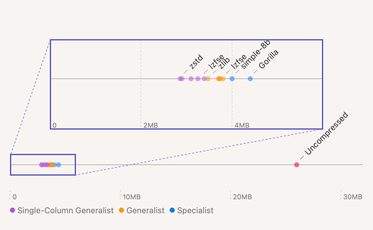
I’ve plotted everything side-by-side:

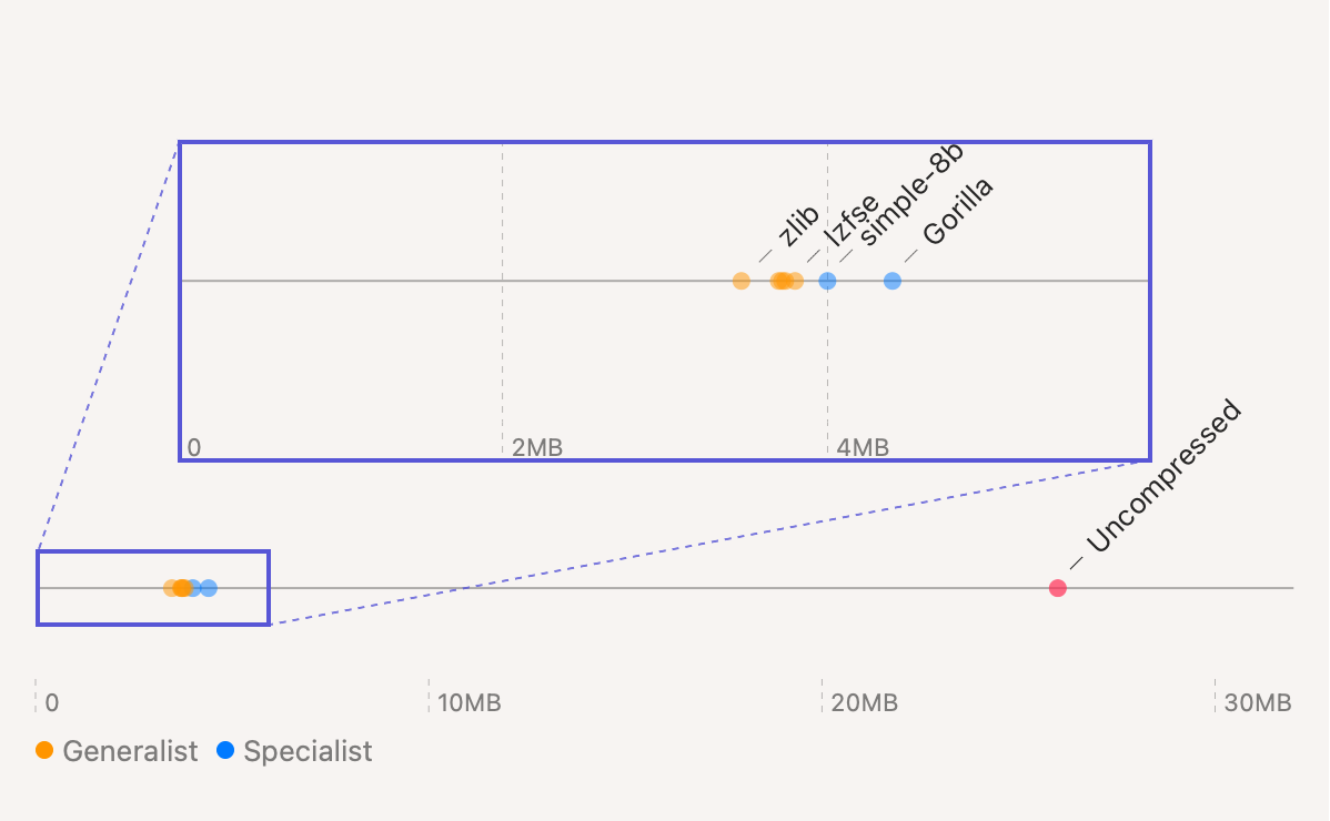_{MB/year by algorithm}

Weirdly, the generalist algorithms universally beat the specialists. On top of that, you’ll recall we picked generalist levels that were fairly fast. So we can actually widen the gap if we’re willing to compress slower.

That feels like cheating, but doing the single column CSV doesn’t. Plus I’m really curious about that, so here it is:

_{MB/year by algorithm including single
column
CSV
results}

Seems like if you’re not a CSV purist you can squeeze an extra 400KB or so. Not bad.

What Gives?

It really does not make sense to me that the generalist algorithms come out on top.

It’s possible I made a mistake somewhere. To check this, I look to see if every compressed time series can be reversed back to the original scale time series. They all can.

My second guess is that maybe my time series data is not well-suited for simple-8b and Gorilla. I saw mention that equally spaced timestamps are preferred and my data is anything but:

`timestamps`	`deltas`
`1691685057323 1691685057413 1691685057504 1691685057622 1691685057732`	`n/a 90 91 118 110`

To see if this is the problem, I re-run the benchmarks and truncate timestamps to the nearest 0.01s, 0.1s and even 1s. This ensures that there is a finite sized set of delta values (101, 11 and 2 respectively).

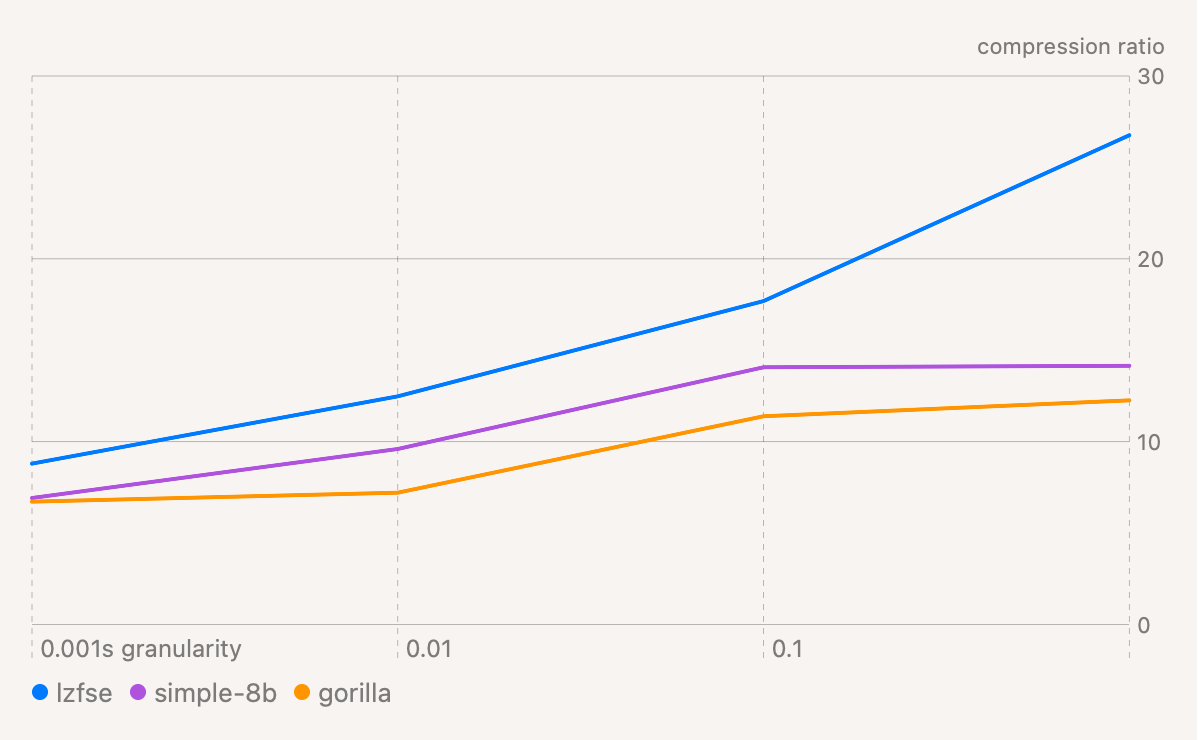_{Compression ratio by timestamp
granularity}

As expected this does improve the compression ratio of the specialist algorithms. But it also gives a similar boost to the generalist one. So it doesn’t explain the difference.

I don’t have a third guess. Maybe it is real?

Back to Where We Started

This all started since I was anxious about inflating the size of my humble iOS app. Our baseline was adding 26MB of new data each year, which became ~100MB/year in iCloud. With a general purpose compression algorithm it looks like we can get these numbers down to ~4MB and ~16MB per year respectively. Much better.

Any of the generalist algorithms would work. In my case using one of Apple’s built-ins is an easy choice:

It’s ~1 line of code to implement them. ^{Plus a few lines to make a CSV.}
Using Brotli or zstd would increase my app’s download size by 400-700 KB. Not a lot but avoiding it is nice.

Try It at Home

One thing we didn’t touch on is that the distribution of your data can impact how well the compression works. It’s possible these results won’t translate to your data. To help check that, I’ve put my benchmarking CLI tool and a speed-test macOS/iOS app up on GitHub here.

If you can put your data in CSV format, you should be able to drop it in and try out all the algorithms mentioned in this post. If you do, let me know what sort of results you get! I'm curious to see more real-world data points.