LLMs for your iPhone: Whole-Tensor 4 Bit Quantization
Shrinking models for Apple Silicon • March 6, 2024Quantization is often touted as a way to make large language models (LLMs) small enough to run on mobile phones. Despite this, very few of the latest methods are able to use the full power of Apple Silicon on iPhone and Mac. This post introduces a new method of quantization that can.
This method is compatible with all three Apple Silicon co-processors (CPU, GPU, Neural Engine) which allows it to take full advantage of the speed/battery trade-offs offered by the hardware.
When compared to standard 4 bit Apple Silicon-compatible methods, it produces consistently more accurate results. Additionally it approaches the accuracy of GPTQ, a widely-used method that is not compatible.
Finally, this method is comparatively accessible. Access to Colab free tier and an Apple Silicon MacBook is sufficient to quantize the full family of GPT-2 models up to 1.5B parameters.
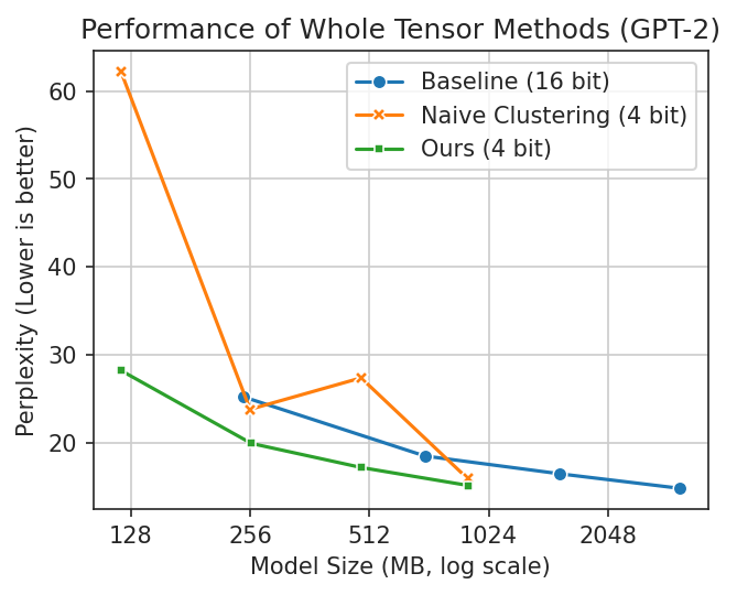
 Lower is better in these plots. You want
a
smaller model with better performance (lower perplexity is better). In the first plot, naive clustering
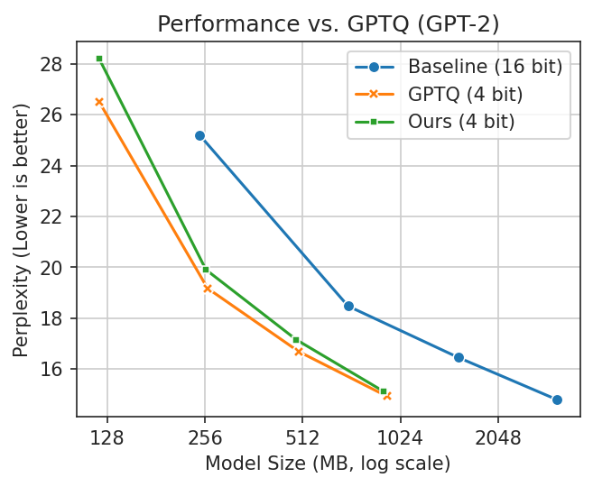
occasionally performs well but is erratic. In the second, GPTQ is better but cannot run fully on Apple
Silicon.
Lower is better in these plots. You want
a
smaller model with better performance (lower perplexity is better). In the first plot, naive clustering
occasionally performs well but is erratic. In the second, GPTQ is better but cannot run fully on Apple
Silicon.
Acknowledgements
This method extends SqueezeLLM, and remixes ideas from both SmoothQuant and AWQ. It was developed concurrently with OneBit, and shares some similar ideas. Thank you for sharing your research and code!
LLM and Quantization Primer
When you ask an LLM a question, that text gets transformed into a matrix of numbers. This matrix is then transformed repeatedly with a bunch of math until a final transformation that converts it from numbers to the first few characters of the LLM's response.
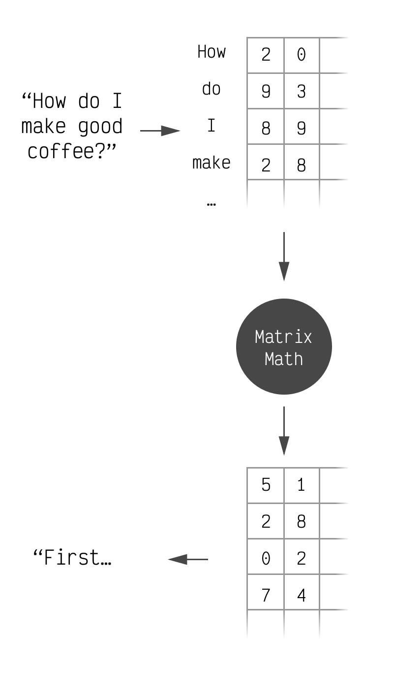 This is accurate for our purposes.
Within these repeated transformations there are many times where the input matrix is multiplied with different hardcoded matrices. These hardcoded matrices can be quite large and end up accounting for most of the space that an LLM takes up. For instance LLaMa 7B, Facebook's open-source LLM, is 13.5GB and 12.9GB of that is the numbers that make up these large matrices.
Typically the matrix's values are stored as 16 bit 2 byte or 32 bit 4 byte floating point numbers. For LLaMa a typical matrix is 4096x4096 which means it takes 33MB on its own. Shrinking those 16 bit elements to 4 bits brings the size of that matrix to 8.3MB. Doing the same for every matrix brings the whole model from 13.5GB to just under 4GB.
Instead of measuring this compression in bytes-per-matrix, it is measured in bits-per-element. (1 byte = 8 bits). This makes it easier to compare across matrices of different sizes and also gives us some flexibility to store a few extra values alongside our matrix. This is actually fairly common. Including them in the bits-per-element calculation makes for fair comparisons.
So, in summary, LLMs do a bunch of math with matrices in order to generate replies. These matrices are big and quantization's goal is to make them smaller without losing the LLM's ability to reply. This shrinks the model and lets us run it on less powerful devices, like your phone.
Challenges with Apple Silicon
If you take the weight from a linear layer (one of the matrices we talked about above) out of an LLM and look at the distribution of its elements, you will generally see a bell curve.
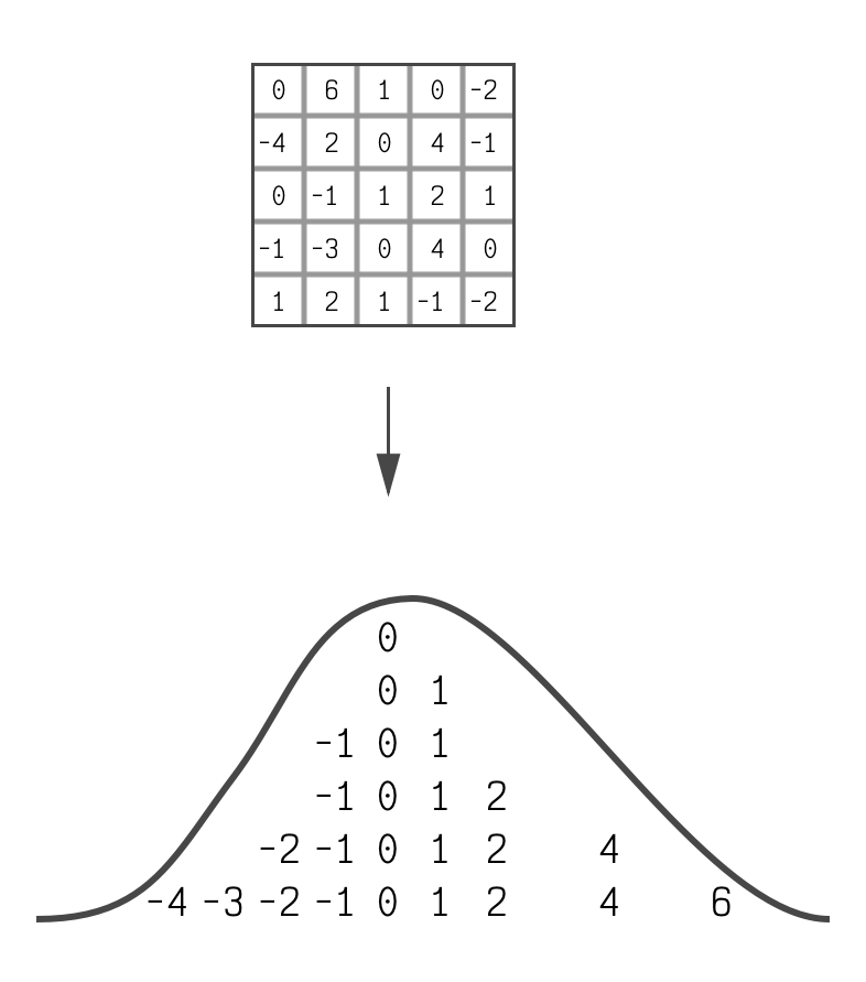 It's not a perfect bell curve, but it's
close enough to be useful.
It's not a perfect bell curve, but it's
close enough to be useful.
Nearly all recent quantization schemes are uniform which means they take this bell curve and pick two values for it. They pick a starting point and also a step size which they then use to place equally-spaced points along the x-axis. To actually quantize the matrix they simply snap all matrix elements to the nearest point.
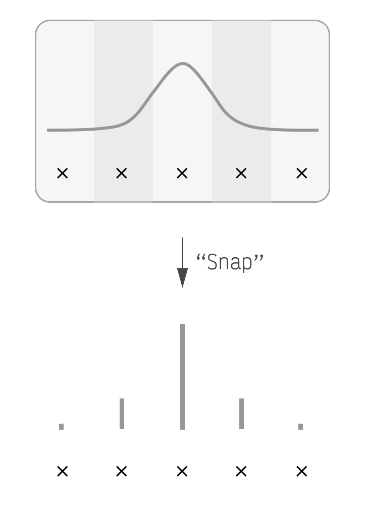 The x points are equally
spaced.
The x points are equally
spaced.
This is a non-optimal use of space in our quantized linear layer. The points on the edges of the bell curve barely capture any matrix elements, but they consume the same amount of space in the LLM as points in the middle which represent many. They are simply not an effective use of bits. (This is fast on GPUs though which is why everyone uses them.)
A common solution for this is to break up the matrix into chunks of either rows, columns, or groups. Having fewer elements in a chunk tends to make quantization more accurate by narrowing the bell curve (more or less) and it only costs a few extra fractions of a bit on average. This sufficiently minimizes the awkwardness of fitting equally-spaced points to bell curve-distributed matrix elements.
Unfortunately Apple Silicon does not support this chunking concept for low (<8) bit quantization. However it makes up for it by allowing models that use a non-uniform quantization scheme. On our bell curve from before, this means we can place our points anywhere we want. So we'll place them optimally.
What is optimal? For each matrix element we calculate how far it is from the nearest point. This is the element's quantization error. We place our points along the bell curve so that the sum of all elements' errors is as low as possible. (k-means clustering is a good way to do this.)
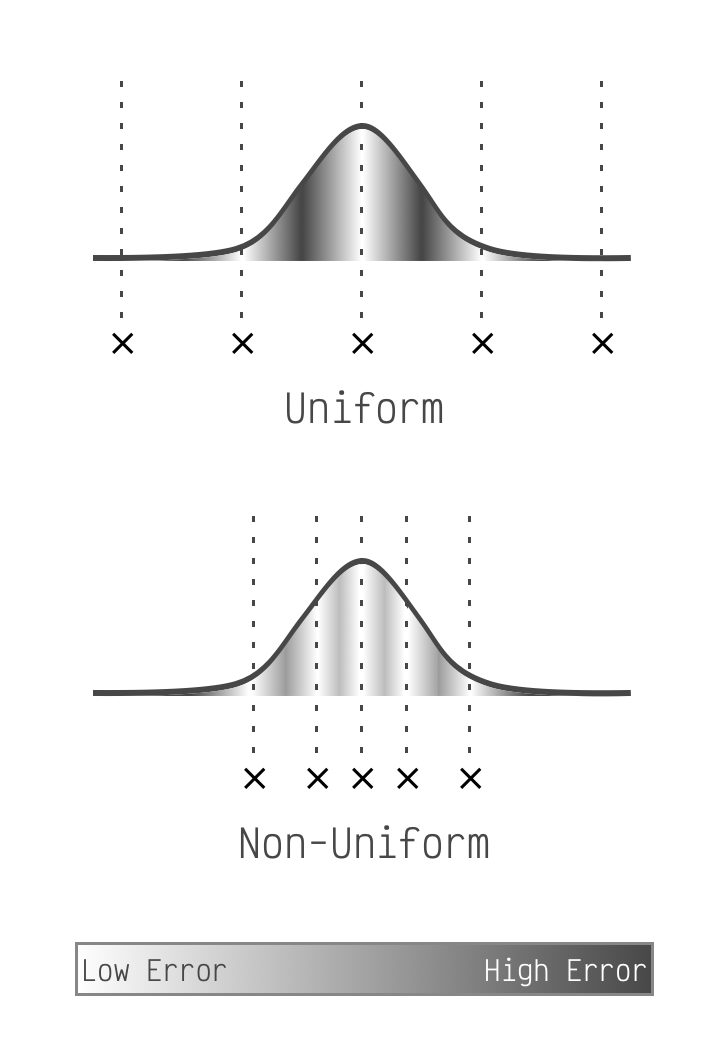 Notice how uniform puts points at the edges,
but non-uniform is free to ignore the small number of matrix elements there.
Notice how uniform puts points at the edges,
but non-uniform is free to ignore the small number of matrix elements there.
Placing the points optimally like this is all we need to do when we have a lot of points to place. Most LLMs will perform very well if we place 6 bits or 8 bits worth of points (64 and 256 respectively). However when we drop to 4 bits worth, which is only 16 points, this simple optimal placement is not enough.
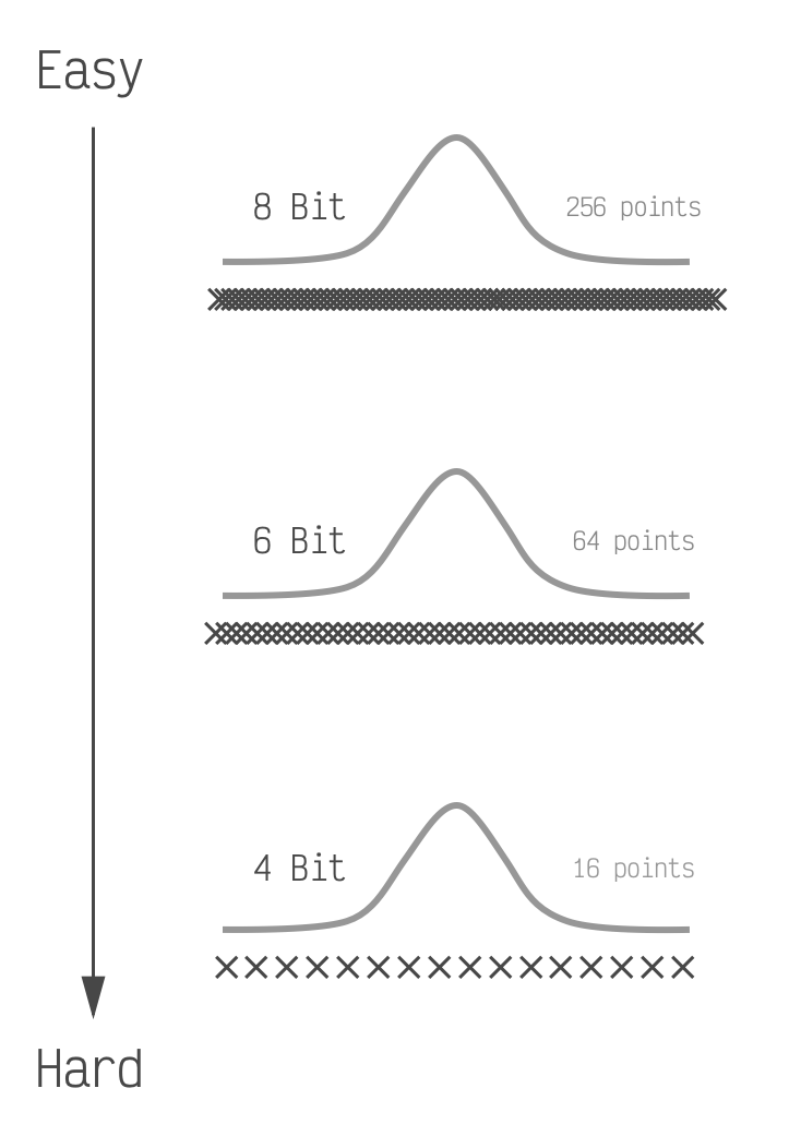 If we were to shade these to show the error
they would get darker going from top to bottom. The LLM performance also typically goes from nearly perfect,
to good, to bad going from top to bottom.
If we were to shade these to show the error
they would get darker going from top to bottom. The LLM performance also typically goes from nearly perfect,
to good, to bad going from top to bottom.
Method Overview
Our goal is to improve LLM performance when using 4-bits as much as possible. We achieve this by making 3 complementary modifications to the quantization process and the LLM itself.
Modification 1: Weighting by Importance
The first modification comes directly from another paper, SqueezeLLM. The paper is fairly approachable, but we'll summarize the parts we're using.
It turns out that every element in these matrices is not equally important. In fact the top few percent are significantly more important. When we're placing our points optimally we should not treat every element equally, but let the more important elements have more sway. But how do we know what's important? We take a small number of input texts (100 is enough), send them through our LLM, and observe the impact each matrix element had on the LLM's response. The higher the total impact, the more important.
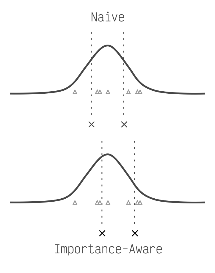 The triangles represent more important
elements. The Naive method is optimal for a standard bell curve, but the importance aware method shifts
closer to the triangles.
The triangles represent more important
elements. The Naive method is optimal for a standard bell curve, but the importance aware method shifts
closer to the triangles.
Modification 2: Scaling for Easier Clustering
So far we've been looking at our matrix as a single bell curve. A different way of thinking about it is to look at every column of the matrix as an independent entity that just happens to be joined together in this matrix. Similar to the matrix as a whole, each column's elements are roughly bell curve-shaped. Most of the bell curves have similar centers but they all have different standard deviations (how wide or narrow they are).
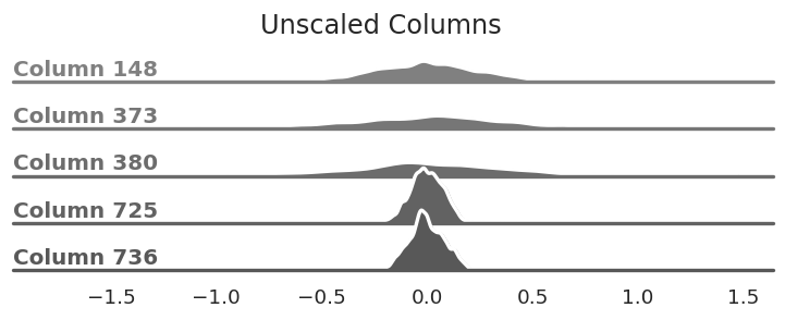 The columns of our matrix are all centered
around zero, but the standard deviation varies—some are very wide while others are fairly
narrow.
The columns of our matrix are all centered
around zero, but the standard deviation varies—some are very wide while others are fairly
narrow.
If we divide the elements of each column by the column's standard deviation we make the bell curves roughly the same shape. This makes it easier to place our points since it prevents one column from having undue influence over the rest. (You can also think of it as squishing more elements towards the middle of the curve where we typically place more points.)
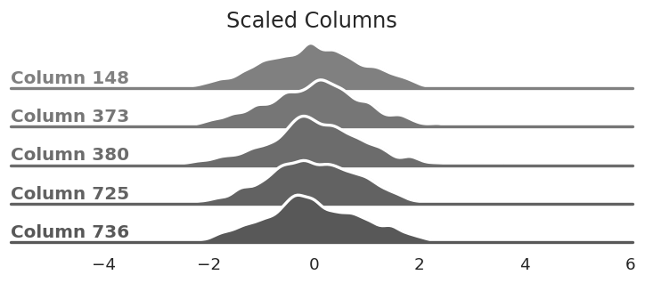 The same columns from above after dividing
every element by each column's standard deviation. This reshapes the bell curves.
The same columns from above after dividing
every element by each column's standard deviation. This reshapes the bell curves.
It's important that we don't change the output of our LLM, and scaling each column independently changes it. So we need to take the per-column values that we divided by and correct for them somewhere else in our model. All of the matrices that we're quantizing are used in matrix multiplications. Since we divide each column, and columns determine the output of the matrix multiplication, we can add a step in our LLM after the multiplication to re-multiply the removed values back in.
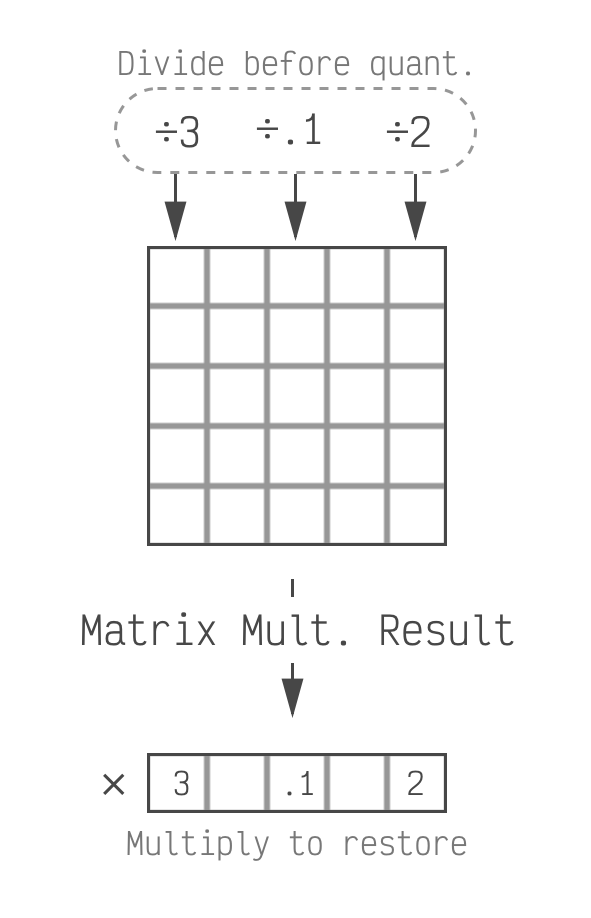 We divide before quantizing which makes
quantization easier. We have to restore the scale factors at inference time, when the model is generating a
response.
We divide before quantizing which makes
quantization easier. We have to restore the scale factors at inference time, when the model is generating a
response.
This does mean we have to keep a few extra values as 16 bit (the ones we multiply back in). For a 768x768 matrix, we need 768 extra values in 16 bits. This puts us at 4.02 bits on average which is a reasonable trade-off. The average number of bits decreases as the model and matrices get larger which makes this even less of a concern. (LLaMa is 4.003 or less depending on the version.)
Modification 3: Shifting the Other Matrix
So far we've been looking closely at the matrix itself. Let's now look at how it is used. As mentioned
above, these matrices are used for matrix multiplication. Specifically the model is performing matrix X
times matrix W, X*W, and we are quantizing W. We've talked about how the elements in W are
nicely distributed with an average close to zero and bell-shaped. This is not true for X. X depends on the
text
that the model received as input and can vary significantly in how its elements are distributed.
Why does this matter? Imagine a simple product of two numbers: x*w. Let's say that in this
case our 1 element matrix, w, has the value of 2.3 and we quantize it to 2. When we do x*2 we
get a quantization error of x*0.3. The closer that x is to zero, the less error. The farther
it is from zero the more we get.
This extrapolates to matrix multiplication. When we look at a column of matrix X, if most of its values are far from zero then the impact of quantization error for that column will be larger.
Similar to our first modification, we can inspect a small number of texts as they flow through the LLM. If we do this we'll see that there is consistency in which columns of X, the input matrix, have larger or smaller values in general.
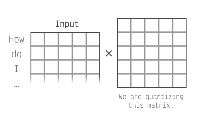 We're focusing on the columns of the left
matrix. This matrix is derived from the input to the LLM.
We're focusing on the columns of the left
matrix. This matrix is derived from the input to the LLM.
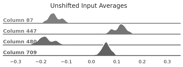 The distribution of average values for
select columns. Notice that they are not centered at zero unlike the matrix we're quantizing.
The distribution of average values for
select columns. Notice that they are not centered at zero unlike the matrix we're quantizing.
To minimize the impact of large values in X we can apply a per-input column shift. This will move most of the values in X closer to zero on average, thereby reducing the impact of our quantization error. We shift by subtracting the average of the values we saw for that column.
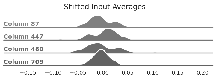 The same columns from above after
subtracting the average value from each column. They are now centered around zero.
The same columns from above after
subtracting the average value from each column. They are now centered around zero.
Similar to our second modification, we need to reverse this change in the model in order to not change its
outputs. This one is a little trickier, but again easier to think about without matrices involved. If we
take our x*w from earlier we can make a new shifted input y (so, y=x-shift). Now
the model will do y*w which is actually (x-shift)*w. If multiply that out we get
x*w - shift*w. Since shift and w are both constants we just need to pre-compute that value and
subtract it after the matrix multiplication in the model. This undoes the impact of shifting X but reduces
the error when w is quantized. (Extrapolating this to matrices is a little harder, but still doable.)
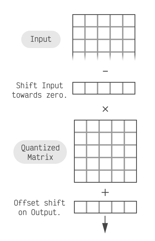 In this case we don't subtract the shift
values themselves, but the result of multiplying all the shifts by the matrix we're quantizing.
In this case we don't subtract the shift
values themselves, but the result of multiplying all the shifts by the matrix we're quantizing.
Depending on the model this adds between zero and two additional vectors of 768 elements in 16 bits. At a worst case this brings us up to 4.06 bits total.
Results
Used individually, these modifications have varying efficacy. Generally the first modification, from SqueezeLLM, works well on its own. When we add in the other two modifications we see consistent improvement. This leaves us with a quantization scheme that is both more accurate and less erratic than the baseline 4-bit method we wanted to improve upon.
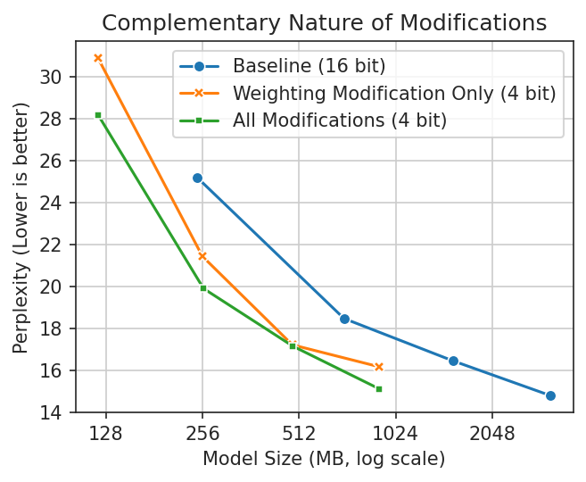 SqueezeLLM (Weighting) is surprisingly
effective on its own, even at the whole-tensor level. Adding our other modifications consistently improves
upon it. The improvement for gpt2-large is negligible—something interesting to follow up on.
SqueezeLLM (Weighting) is surprisingly
effective on its own, even at the whole-tensor level. Adding our other modifications consistently improves
upon it. The improvement for gpt2-large is negligible—something interesting to follow up on.
Conclusion
tl;dr We used an amalgamation of existing and, I think, new ideas to quantize LLM linear layers to ~4 bits on average, dramatically shrinking model size. Since we do this at the tensor level without grouping, this method is fully compatible with Apple Silicon on iPhone or Mac which opens the door for larger models on your devices.
Thanks for reading! To stay in the loop as I explore more, you can give me a follow on Twitter. If you'd like to give it a go yourself, I've got a drop-in replacement for torch's Linear layer, as well as some instructions: here. Please get in touch, ask questions, and let me know what you learn!
Appendix: Future Ideas
Part of my motivation for writing this is to find folks who are smarter than me, who can maybe check my work, and maybe even take it further. If that's you, do please reach out! There's a couple directions that I think still have more to give / would be interesting to explore:
- I couldn't find a way to scale the input channels (weight matrix rows) that was helpful. Seems like there might be something there, either as a way to make clustering easier, or as a way to minimize error from the inputs.
- Depending on the model, sometimes computing a weighted standard deviation based on the SqueezeLLM sensitivities performs slightly better. This makes me think that standard deviation is close but not the optimal solution.
- These models seem very reactive to how the SqueezeLLM sensitivities are generated. I suspect any improvements there would help.
- Explore integrating this with Mixed Bit Precision methods.
Appendix: Modification Comparison
To further support that these modifications are complementary, wikitext perplexity was measured in all possible combinations. As mentioned above, gpt2-large is an outlier but the differences are minor. The SqueezeLLM fisher information (sensitivities) were computed using C4 in all cases.
| Model | Weighting | Scaling | Shifting | Weight+Scale | Weight+Shift | Scale+Shift | Weight+Scale+Shift |
|---|---|---|---|---|---|---|---|
| gpt2 | 30.8947 | 43.0891 | 44.9285 | 28.8972 | 29.1401 | 43.5065 | 28.1946 |
| gpt2-medium | 21.4389 | 30.9959 | 23.8464 | 20.4853 | 19.8515 | 23.6801 | 19.904 |
| gpt2-large | 17.2172 | 22.5075 | 18.1454 | 17.1246 | 17.1282 | 25.2589 | 17.1507 |
| gpt2-xl | 16.1751 | 15.89 | 15.7223 | 15.148 | 16.0874 | 17.0936 | 15.1148 |
| Model | float16 | naive 4-bit | Weight+Scale+Shift | GPTQ |
|---|---|---|---|---|
| gpt2 | 25.1876 | 62.1889 | 28.1946 | 26.5 |
| gpt2-medium | 18.4739 | 23.7826 | 19.904 | 19.1719 |
| gpt2-large | 16.4541 | 27.3636 | 17.1507 | 16.6875 |
| gpt2-xl | 14.7951 | 15.89 | 15.1148 | 14.9297 |